TEXSTAN

Institut für Thermodynamik der Luft- und Raumfahrt - Universität Stuttgart
Mechanical Engineering - The University of Texas at Austin

TEXSTAN Input Variables - definitions and explanations

Within this section are the definitions of the flags and variables that appear in an input dataset for TEXSTAN. The section glossary contains definitions and explanations of terms that are often used in convective heat, mass, and momentum transfer. Definitions of the variables that appear in the output files are found in external flows: output files and internal flows: output files sections of this website.

A B C D E F G H I J K L M N O P–Q R S T U V W X Y–Z

###
1	title
2	kgeom	neq	kstart	mode	ktmu	ktmtr	ktme
3	kbfor	jsor(1)	jsor(2)	jsor(3)	jsor(4)	jsor(5)
4	kfluid	kunits
5	po	rhoc	viscoc	amolwt	gam/cp
6	prc(1)	prc(2)	prc(3)	prc(4)	prc(5)
7	nxbc(I)	jbc(I,1)	jbc(I,2)	jbc(I,3)	jbc(I,4)	jbc(I,5)
8	nxbc(E)	jbc(E,1)	jbc(E,2)	jbc(E,3)	jbc(E,4)	jbc(E,5)
9	x(m)	rw(m)	aux1(m)	aux2(m)	aux3(m)
9	ubI(m)	am(I,m)	fj(I,1,m)	fj(I,2,m))	fj(I,3,m)	fj(I,4,m)	fj(I,5,m)
10	ubE(m)	am(E,m)	fj(E,1,m)	fj(E,2,m))	fj(E,3,m)	fj(E,4,m)	fj(E,5,m)
11	xstart	xend	deltax	fra	enfra
12	kout	kspace	kdx	kent
13	k1	k2	k3	k4	k5	k6
14	k7	k8	k9	k10	k11	k12
15	axx	bxx	cxx	dxx	exx	fxx	gxx
16-ext	dyi	rate	tstag	vapp	tuapp	epsapp
16-int	dyi	rate	reyn	tref	tuapp	epsapp	twall

A top of page

am(E,m)

am(E,m)	kgeom	definition
= 0.0	= 1,2,3	not an option (this is entrainment)
= 0.0	= 4,5,6,7	not an option

For external flows (kgeom=1,2,3) there is technically a mass transfer at the E-surface, and it is called entrainment. This is primarily because external flows are contained by a well-defined boundary (the I-surface, a wall) and an ill-defined "infinity" boundary (the E-surface, or free stream). Boundary layer flows (external flows) have to have special handling for the infinite boundary condition to insure that all dependent variable gradients approach zero as the dependent variables approach their free stream values. Control of the E-surface mass flux (entrainment) helps to assure the zero gradient condition by moving the E-surface. Without entrainment, the free stream value will be forced, but the gradient will be non-zero, and the overall numerical solution will be completely incorrect. We use benchmark data sets to ensure that TEXSTAN's entrainment model is correct. In contrast, internal flows have both their I- and E-surfaces well defined, and entrainment does not exist. Entrainment is discussed in the Entrainment Control and Entrainment Theory parts of external flows: integration control sections of this website.

The am(E,m) array values are set =0.0 for both internal and external flows because E-surface mass flux can not be prescribed as a boundary condition. Note that the array values can not be left blank because they are part of the structured data input for TEXSTAN.

am(I,m)

am(I,m)	kgeom	definition
= m_s"(x)	= 1	wall transpiration at the I-surface, (units of kg/m², SI; lbm/ft², US/Eng)
= 0.0	= 2,3 and 4,5,6,7	not an option

This boundary condition array provides wall mass flux (cross-stream or y-directed mass flux), called transpiration in boundary layer theory. The value is positive for blowing (mass flux injected into the boundary layer) and negative for suction (mass flux removed from the boundary layer). Transpiration really only works in TEXSTAN for kgeom=1. The definition is related to the blowing fraction: F = (ρv)_s / (ρv)_∞ . For blowing the limit is typically F=0.01, and for larger values the flow separates from the surface.

amolwt

Fluid molecular weight (units are kg/(kg-mole) or (kg/kmol), SI; lbm/(lbm-mole) or lbm/(lbm-mol), US/Eng)

amolwt	kfluid	molecular weight
= 0.0	=1	not required
= 0.0	= 4,16	not required
= 0.0	= 2,6,8	set by fluid within tables
= M (input variable)	= 14,15

aux1(m)

aux1(m)	definition
deltax	nondimensional integration stepsize

This variable array is used in conjunction with kdx=1 to provide integration stepsize information using the array aux1(m) which is then linearly interpolated as a function of x. If kdx is set =1, then deltax is set =0.0. This variable is rarely used for external boundary layer flows except to resolve surface temperature (or) heat flux in the vicinity of a step change in the thermal boundary condition. Use of aux1(m) in place of deltax is really mandatory for combined entry flow in pipes and channels that begin with flat profiles for velocity and temperature, for both laminar and turbulent flows (especially with two-equation turbulence models). It is also needed for the unheated starting length flow heat transfer problem. The recommended distribution of stepsizes for internal flows is presented in the integration stepsize part of the internal flows: integration control section of this website.

aux2(m)

aux2(m)	definition
(r_o - r_i)	distance between the outer and inner radius (kgeom=7); units are m, SI; ft, US/Eng
S	volumetric energy source, jsor(j)=5,6,7,8; units are J/m³, SI (or) Btu/ft³, US/Eng

For the annular geometry, the annular gap (distance between the outer and inner radius) is not allowed to change with x. Note that for an annulus, the hydraulic diameter is twice the gap width.

For the volumetric energy source, there is no distribution with y in academic TEXSTAN.

aux3(m)

aux3(m)	definition
X	volumetric momentum body force, kbfor=3,4; units are N/m³, SI (or) lbf/ft³, US/Eng
R	surface axial radius of curvature, kbfor=5; units are m, SI (or) ft, US/Eng

For the volumetric momentum body force , there is no distribution with y in academic TEXSTAN.

The surface radius of curvature is used in conjunction with the mixing length turbulence model as described in the modeling: curvature section of this website. The aux3(m) array is linearly interpolated to obtain R(x).

It is imperative that this distribution be smooth, and it can be checked using the k8=36 diagnostic check, as discussed in the overview: bc smoothness section of this website. To generate this file TEXSTAN takes the input variables that define the integration starting x location (xstart) and stopping x (xend) location and subdivides the interval into 250 equally spaced values. It then interpolates the array aux3(m) using linear interpolation to obtain these 250 locations. The results are written into a file called tex_wall.txt. Plotting the resulting R(x) array in this file will help you see if your input wall radius distribution is smooth enough. If it is not, you may want to slightly move some of the points or re-smooth the array using software that smooths experimental data, such as a least-squares spline-with-tension package.

axx

axx	definition
κ	mixing length model constant (ktmu=2,8) see modeling: mixing-length model
a	model coefficient (units of m/s, SI, (or) ft/s, US/Eng) in the analytical velocity model for the 2-D stagnation point flow (k4=5) see k4
V_app	approach velocity (units of m/s, SI, (or) ft/s, US/Eng) in the analytical velocity model for the cylinder-in-crossflow (k4=6) see k4
Re_δ2	transition momentum Reynolds number for the Lam-Bremhorst two-equation model (ktmtr=2) see modeling: transition

B top of page

bxx

bxx	definition
λ	mixing length model constant (ktmu=2,8) see modeling: mixing-length model
b	model coefficient (units of m, SI, (or) ft, US/Eng) in the analytical velocity model for the 2-D stagnation point flow (k4=5) see k4
R	cylinder radius (units of m, SI, (or) ft, US/Eng) in the analytical velocity model for the cylinder-in-crossflow (k4=6) see k4
Re_x	x-Reynolds number for use with flag k10=21 see k10
Re_δ2	momentum thickness Reynolds number for use with flag k10=22 see k10
Re_Δ2	enthalpy thickness Reynolds number for use with flag k10=23 see k10
x/D_h	x normalized by the hydraulic diameter for use with flag k10=24 see k10
intg	integration step for use with flag k10=25 see k10

C top of page

cxx

cxx	definition
A⁺	mixing length model constant (ktmu=2,8) see modeling: mixing-length model
c	model coefficient (units of m, SI, (or) ft, US/Eng) in the analytical velocity model for the 2-D stagnation point flow (k4=5) see k4
k_s	roughness height (units of m, SI, (or) ft, US/Eng) for the E-surface (kgeom=4,5,6,7)in the mixing length roughness model, see modeling: roughness

D top of page

deltax

deltax	integration stepsize
> 0.0	nondimensional variable that is used to calculate integration step size
= 0.0	integration stepsize being controlled by flag kdx =1 and array aux1(m)

Note: when flag kdx =1, the deltax variable must be set =0 because of the way the TEXSTAN's input file read structure is designed, even though entrainment is not applicable for internal flows.

For external flows, the nondimensional stepsize is the fraction of velocity boundary layer 99% thickness, and for internal flows it is a fraction of the pipe radius, or channel half width, or average annulus radius. These definitions hold regardless of whether the stepsize is input using deltax or using the aux1(m) array.

For external flows, the numerical grid extends only from the surface to just above the shear layer (boundary layer). This is usually called the free stream. For external flows TEXSTAN's integration stepsize is proportional to the boundary layer thickness, so as the boundary layer grows, the stepsize automatically increases. The primary input variable for stepsize control is deltax. We typically set deltax =0.05 to =0.10, and this works well for most laminar, transitional, and turbulent flows. However, the integration stepsize must be kept smaller to resolve fast-changing boundary conditions. A more detailed discussion of stepsize can be found in the external flows: integration control section of this website.

For internal flows, the numerical grid is required to extend from the surface to the centerline for pipes and thermally-symmetrical parallel-planes channels (kgeom=4,5) or from surface to surface for thermally-asymmetrical parallel-planes channels and annuli (kgeom=6,7). As with external flows, we typically set deltax =0.05 to =0.10, and this works well for pipe and channel flows once the developing shear layer (boundary layer) diffuses to the pipe or channel centerline. However, the integration stepsize must be kept much smaller to resolve the entry flow where the shear layer starts with zero thickness.

The combined entry flow in pipes and channels begin with flat profiles for velocity and temperature, so the developing shear layer (boundary layer) is a really a very small percentage of this grid in the beginning. If deltax is set small enough to resolve the extremely high wall gradients in the beginning part of the entry region, the total number of integration steps will be massively large by the time the entry flow is complete and fully-developed flow begins. Instead of using deltax we set the flag kdx =1, set deltax =0, and input deltax information using the array aux1(m) which is then linearly interpolated as a function of x . This is why the user will see a peculiar x(m) distribution, and the small aux1(m) values near x=0. The actual integration stepsize becomes proportional to the interpolated aux1(m) array, =aux1*yl , where yl is the pipe radius, half-width of a parallel-planes channel, or the average of the inner and outer radii for an annulus. A more detailed discussion of stepsize can be found in the internal flows: integration control section of this website.

dxx

dxx	definition
a	model coefficient in the ε_M constant diffusivity model constant (ktmu=8) see modeling: mixing-length model
d	model coefficient in the analytical velocity model for the 2-D stagnation point flow (k4=5) see k4

dyi: The variables dyi and rate set the y spacing for the velocity profile, which in turn controls the grid (finite difference mesh) for TEXSTAN. These variables are explained in considerable detail in the external flows: initial profiles and internal flows: initial profiles sections of this website.

E top of page

enfra

enfra	flag to control entrainment
= 0	internal flows (not applicable)
> 0	external flows

Note: for internal flows, enfra must be set =0 because of the way the TEXSTAN's input file read structure is designed, even though entrainment is not applicable for internal flows.

The enfra variable is part of the set of variables used to control entrainment for external flows. The set also includes fra and kent, and a discussion of entrainment can be found in the external flows: integration control section of this website. The suggested values for external flow are

enfra	nondimensional variable to trigger calculation of entrainment for external flows
1.0E-06	recommended value for flat plate geometry external flows
1.0E-04	recommended value for turbine blade geometry external flows

For external flows (kgeom=1,2,3) there is technically a mass transfer at the E-surface, and it is called entrainment. This is primarily because external flows are contained by a well-defined boundary (the I-surface, a wall) and an ill-defined "infinity" boundary (the E-surface, or free stream). Boundary layer flows (external flows) have to have special handling for the infinite boundary condition to insure that all dependent variable gradients approach zero as the dependent variables approach their free stream values. Control of the E-surface mass flux (entrainment) helps to insure the zero-gradient condition by moving the E-surface. In TEXSTAN the surface movement is automatic because of the nature of the transformed variables that utilize the von Mises stream function. Note that for other types of finite-difference programs, the computations have to be stopped, a new mesh constructed, and the variable values interpolated onto the new grid, before integration can continue. Without entrainment, the free stream value will be forced, but the gradient will be non-zero, and the overall numerical solution will be completely incorrect.

The overall entrainment procedure at each integration step is to compute the near-edge gradient of each dependent variables within the set of variables defined by the value of kent. For example, kent=0 requires only the edge velocity gradient to be tested, and kent=1 requires additional testing of the temperature (or stagnation enthalpy) profile. Each tested gradient is then made nondimensional and compared with the value of enfra. If the absolute value of any tested gradient exceeds the enfra value, an algorithm computes an incremental E-surface mass flux and adds it to the existing E-surface value. The incremental mass flux is then tested against the fra value and limited to the fra value.

We use benchmark data sets to ensure that TEXSTAN's entrainment model is correct. In contrast, internal flows have both their I- and E-surfaces well defined, and entrainment does not exist. Entrainment is discussed in the Entrainment Control and Entrainment Theory parts of the external flows: integration control section of this website.

epsapp

approach turbulence dissipation or inlet turbulence dissipation (units are m²/s³, SI; ft²/s³, US/Eng)

epsapp	ktmu	turbulence dissipation, for use with internal and external flow turbulence models
= 0.0	= 1-8	not required for mixing-length models
= 0.0	= 11	not required for the one-equation model
= ε_app	= 21-24	required for external flow two-equation turbulence models
= ε_inl	= 21-24	required for internal flow two-equation turbulence models

For external flows the initial edge value ε_inl,∞ is either equated to the input variable epsapp (providing its value is > 0.001), or it is computed within TEXSTAN if the input value of epsapp is set =0. The internally computed value using a model based on the two-equation formulation of the turbulent viscosity eps,inf initial value formulation
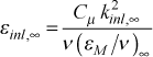
Note, if epsapp is given a value on the order of 0.0001-0.001, it will prevent the free stream turbulence kinetic energy from changing (creating what is often called "frozen" turbulence). This calculation is presented in the external flows: initial profiles section of this website. Note: for laminar flows and transitional or fully turbulent flows using either the mixing length or the one-equation turbulence model, epsapp must be set =0 because of the way the TEXSTAN's input file read structure is designed.

For internal flows the initial value ε_inl at the inlet to the pipe or channel is either equated to the input variable epsapp (providing its value is > 0.001), or it is computed within TEXSTAN if the input value of epsapp is set =0. The internally computed value using a model based on the two-equation formulation of the turbulent viscosity inlet dissipation formulation
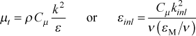
Note, if epsapp is given a value on the order of 0.0001-0.001, it will prevent the initial turbulence kinetic energy from changing (creating what is often called "frozen" turbulence). This calculation is presented in the internal flows: initial profiles section of this website. Note: for laminar flows and transitional or fully turbulent flows using either the mixing length or the one-equation turbulence model, epsapp must be set =0 because of the way the TEXSTAN's input file read structure is designed.

exx

exx	definition
b	model coefficient in the ε_M constant diffusivity model constant (ktmu=8) see modeling: mixing-length model
s	scaling coefficient (units of m, SI, (or) ft, US/Eng) to convert x to x/s, mostly for the ftn files (k5 > 0 or k8=36), see external flows: output files or internal flows: output files

F top of page

fj(I,j,m)

boundary condition arrays for the diffusion equations at the I-surface

energy equation I-surface

fj(I,j,m)	kgeom	definition
T_s (x)	1,2,3 and 6,7	surface temperature (units of ºC or K, SI (or) ºF or ºR, US/Eng) note: must use absolute temperature for kfluid>1 (requires jbc(I,j)=1)
q_s" (x)	1,2,3 and 6,7	surface heat flux (units of W/m², SI (or) Btu/(s-ft², US/Eng) (requires jbc(I,j)=2)
= 0.0	4,5	symmetry line boundary condition, ∂T/∂r = 0.0 or ∂T/∂y =0.0 (requires jbc(I,j)=0)

mass transfer equation I-surface

fj(I,j,m)	kgeom	definition
m_j,s" (x)	1	surface mass concentration, m_j = (ρ_j /ρ_mix), (units of kg(j)/kg(mix) SI or lbm(j)/lbm(mix) US/Eng) (requires jbc(I,j)=1) Note: if small mass transfer theory is assumed, the mixture density is constant over the boundary layer, and m_j can be replaced by ρ_j or a concentration variable (c_j M), where M is the molecular weight

turbulence kinetic energy equation I-surface

fj(I,j,m)	kgeom	definition
= 0.0	1,2,3 and 6,7	no-slip boundary condition (all turbulence models) (requires jbc(I,j)=1)
= 0.0	4,5	symmetry line boundary condition, ∂k/∂r = 0.0 or ∂k/∂y =0.0 (all turbulence models) (requires jbc(I,j)=0)

turbulence dissipation equation I-surface

fj(I,j,m)	kgeom	definition
= 0.0	1,2,3 and 6,7	either no-slip boundary condition or zero gradient boundary condition (requires jbc(I,j)=1 for all models)
= 0.0	4,5	symmetry line boundary condition, ∂ε/∂r = 0.0 or ∂ε/∂y =0.0 (all turbulence models) (requires jbc(I,j)=0)

fj(E,j,m)

boundary condition arrays for the diffusion equations at the E-surface

energy equation E-surface

fj(E,j,m)	kgeom	definition
= 0.0	1,2,3	free stream static (or) stagnation temperature - not an option (set =0.0) because temperature will be specified by tstag variable (requires jbc(E,j)=1)
T_s (x)	4,5,6,7	surface temperature (units of ºC or K, SI (or) ºF or ºR, US/Eng) note: must use absolute temperature for kfluid>1 (requires jbc(E,j)=1)
q_s" (x)	4,5,6,7	surface heat flux (units of W/m², SI (or) Btu/(s-ft², US/Eng) (requires jbc(E,j)=2)

mass transfer equation E-surface

fj(E,j,m)	kgeom	definition
m_j,∞"	1	free stream mass concentration (fixed value) (requires jbc(E,j)=1)

turbulence kinetic energy equation E-surface

fj(E,j,m)	kgeom	definition
= 0.0	1,2,3	free stream turbulence kinetic energy - not an option (set =0.0) variable k_∞ initially set by tuapp and then changed according to the turbulence model (requires jbc(E,j)=1)
= 0.0	4,5,6,7	no-slip boundary condition (all turbulence models) (requires jbc(E,j)=1)

turbulence dissipation equation E-surface

fj(E,j,m)	kgeom	definition
= 0.0	1,2,3	free stream turbulence dissipation - not an option (set =0.0) variable ε_∞ initially set by epsapp or internal TEXSTAN model for its initial value and then changed according to the turbulence model (requires jbc(E,j)=1)
= 0.0	4,5,6,7	no-slip boundary condition (all turbulence models) (requires jbc(E,j)=1)

fra

fra	flag to control entrainment
= 0.0	internal flows (not applicable)
> 0.0	external flows

Note: for internal flows, fra must be set =0 because of the way the TEXSTAN's input file read structure is designed, even though entrainment is not applicable for internal flows.

The fra variable is part of the set of variables used to control entrainment for external flows. The set also includes enfra and kent, and a discussion of entrainment can be found in the external flows: integration control section of this website. It places an upper limit on the entrainment, in an attempt to limit excessive boundary layer growth between integration steps, and thus an excessive integration stepsize. The suggested values for external flow are

fra	nondimensional variable to limit entrainment for external flows
0.01	recommended value for external flows

For external flows, the region above the wall that is influenced by the wall boundary conditions varies in the flow direction, and its extent is different for each transport equation (velocity, temperature or stagnation enthalpy, turbulence kinetic energy, and so forth). That is, each equation has its own boundary layer thickness, defined as the location where the dependent variable is within, say, 1 percent of its free stream value. The finite difference computational domain must extend beyond the largest of the boundary layer thicknesses to maintain an overall grid- or finite-difference mesh-independent solution.

Entrainment rarely causes problems, except for the velocity boundary layer in a severe adverse pressure gradient, the velocity boundary layer of a natural convective flow, or the dissipation (and sometimes turbulence kinetic energy) boundary layer of a two-equation turbulence model. With all three, calculated entrainment can be excessively large, causing an artificially large velocity boundary layer thickness, and therefore an integration stepsize that is excessive (recall that the stepsize is proportional to the velocity boundary layer thickness and the proportionality constant is deltax).

For the adverse pressure gradient, the deceleration of the free stream velocity causes the near-edge velocity gradient to change rapidly, and the calculated entrainment that is needed to control the strong change in edge gradient can be large. With the adverse pressure gradient, fra is an attempt to decrease the stepsize (and thus entrainment) as separation approaches. However, if the pressure gradient is strong enough, a zero wall shear stress will eventually occur, causing TEXSTAN to stop.

For the natural convective flow the velocity profile has a large maximum in the near-wall region and then the velocity profile asymptotically approaches a zero gradient far from the wall. The boundary layer thickness is very poorly defined, and the effect of improper entrainment is to create a rather large region of near-zero velocity, which rarely affects the wall stress and heat flux, but is annoying.

A similar issue can arise with the k and ε profiles of the two-equation model. Especially problematic is the ε profile because of the 4-5 orders of magnitude change between the near-wall region and its free stream value, leading to an ill-defined dissipation boundary layer thickness and near-free stream gradient. To control the two-equation model, one solution is to set the kent variable to not include turbulence dissipation in the entrainment testing.

fxx

fxx	definition
Pr_t	turbulent Prandtl number (ktme=2) see modeling: turbulent Prandtl number

G top of page

gam/cp

This is the only input variable in TEXSTAN that has a dual interpretation. It is used to determine the specific heat of the fluid.

the ratio of specific heats for gases (often given the symbol of γ or κ in the classical thermodynamics literature)
c_p, specific heat at constant pressure for gases (units are J/(kg-K), SI; Btu/(lbm-°R), US/Eng)
c, specific heat for liquids (units are J/(kg-K), SI; Btu/(lbm-°R), US/Eng)

gam/cp	kfluid	ratio of specific heats (or) specific heat
= c_p (or) c (input variable)	=1
= 0.0	=2,4,6,8,16	c_p (or) c computed from the i(T) static enthalpy table
= 0.0	=13	computed from c_p(T) correlation
= γ (input variable)	=14,15	c_p will be computed using ideal gas law

Warning: if gam/cp is interpreted as specific heat and SI units are being used, a classical mistake is to input the physical variable using the kJ/(kg-K) (kilojoules version) because this is what is contained in most thermophysical properties tables. TEXSTAN uses J/(kg-K).

gxx

gxx	definition
x_vo	virtual origin (units of m, SI, (or) ft, US/Eng) in the x-Reynolds number for turbulent flow starting profiles (k1=1 and kstart=3), see k1
g	gravitational constant (units of m²/s, SI, (or) ft²/s, US/Eng) for use in the body force term (kbfor=2,4), see kbfor
Re_δ2	transition momentum Reynolds number for the abrupt transition model (ktmtr=1) see modeling: transition
Re_δ2	start of transition momentum Reynolds number (if k9 is set > 0 it replaces the transition start correlation in the Abu-Ghannam and Shaw transition model, ktmtr=3) see modeling: transition
Re_δ2	transition momentum Reynolds number for the Kays and Crawford transition model (ktmtr=4) see modeling: transition
Re_δ2	start of transition momentum Reynolds number (if k9 is set > 0 it replaces the transition start correlation in the Mayle transition model, ktmtr=5) see modeling: transition
k_s	roughness height (units of m, SI, (or) ft, US/Eng) for the I-surface (kgeom=6,7) in the mixing length roughness model, see modeling: roughness
δ	boundary layer thickness or height (units of m, SI, (or) ft, US/Eng) for use with kgeom=1kstart=9 to create flat initial profiles that simulate flow over extremely rough surfaces roughness height (units of m, SI, (or) ft, US/Eng) for the I-surface (kgeom=6,7) in the mixing length roughness model, see modeling: roughness

H top of page

I top of page

J top of page

jbc(E,j): See jbc(I,j) - which contains both definitions.

jbc(I,j)

jbc(I,j)	type of boundary condition at I-surface for each diffusion equation
= 0	symmetry line at the I-surface (applicable only to kgeom=4,5)
= 1	level - T_s , k_s , ε_s at the I-surface
= 2	flux - q_s" at the I-surface

jbc(E,j)	type of boundary condition at E-surface for each diffusion equation
= 0	symmetry line at the E-surface (never used for any kgeom)
= 1	level - T_s , k_s , ε_s at the E-surface
= 2	flux - q_s" at the E-surface

note: the jbc(I,j) and jbc(E,j) entries can be left blank if neq=1 and only the momentum equation is being solved. They can also be left blank for any that are not needed. For example if neq=2, then (neq-1)=1 and TEXSTAN will only read jbc(I,1) and jbc(E,1) .

TEXSTAN has two basic types of thermal boundary conditions that affect the wall temperature and promote heat transfer. The first type controls the wall temperature (the Dirichlet type of boundary condition) and the second type controls the wall heat flux (the Neumann type of boundary condition). In either case, TEXSTAN permits the wall temperature or wall heat flux to vary in the flow direction. A constant wall temperature boundary condition (isothermal) typically models a wall that either has some sort of phase change process occurring on the other side of the wall or the wall has a thermal mass (mass-specific heat product) that is large enough that it can be considered isothermal while exchanging heat with the fluid. A constant heat flux boundary condition typically models a wall that either has some sort of thermal radiation loading onto the wall or there is a heat flux source on the other side of the wall due to Joule heating or a nuclear source.

Each partial differential equation being solved in TEXSTAN must have its type declared for the I- and E- surfaces. The numerical formulation in TEXSTAN makes a clear distinction between solving the momentum equation and solving the various diffusion equations (for example, energy, turbulence variables, mass transfer). The boundary condition type for momentum (Dirichlet for a no-slip surface or free stream and Neumann or zero velocity gradient for a symmetry line). For each diffusion equation the type of boundary condition at each surface must be specified.

jsor(j)

Examples of diffusion equations currently within TEXSTAN include:

i^* , stagnation enthalpy equation (variable properties,kfluid>1)
T , temperature equation (constant properties, kfluid=1)
k , turbulence kinetic energy equation
ε , turbulence dissipation equation
m_j , mass concentration of component A in and A-B boundary layer

and the corresponding jsor(j) values will be

jsor	type of diffusion transport equation
= 1-8	energy equation (stagnation enthalpy (kfluid>1) or temperature (kfluid=1)
= 11	turbulence kinetic energy equation (applicable to either a one-equation model or a two-equation model of turbulence)
= 21	turbulence dissipation equation (applicable to a two-equation model of turbulence)
= 31	mass transfer equation

For example, if jsor(j=1) = 1, the first diffusion equation is an energy equation, and if jsor(j=1) = 11 the first diffusion equation will be a turbulence kinetic energy equation.

The flag jsor(j) is a one-dimensional array directly linked to the value of the variable neq, whose minimum value is =1 and the maximum value is =6. If neq =1 TEXSTAN only solves the momentum equation; otherwise TEXSTAN solves the momentum equation and one or more diffusion transport equations for scalars, as discussed in the definition of the variable neq. There will be (neq-1) diffusion equations if neq > 1. For example, solving the momentum and energy equation will make neq=2, and there will be one diffusion equation. For j=1,(neq-1) TEXSTAN reads the jsor(j) array and compares what it reads for each jsor(j) to a table that translates the element value into what each diffusion equation will be.

The common structure of all the equations (see Generalized Transport Equation in the overview: transport equations section of this website) is reproduced here in the form programmed into TEXSTAN (axisymmetric coordinates) general conv-diff eqn
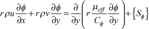
where C equals unity for momentum, and for the various scalar transport equations it represents the appropriate non-dimensional effective transport coefficient. The S_φ term represents the collective of all source and sink terms for the dependent variable in question.

Within the transport equations section is the stagnation enthalpy equation stagnation enthalpy eqn
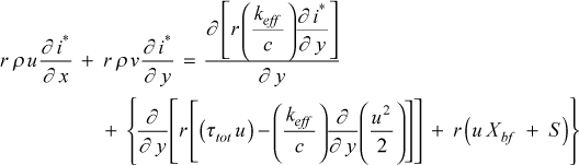
and comparing this equation with the generalized equation, we can see that S_φ is comprised of three terms. The first term is the viscous work term (uτ), the second term is the gravitational work term associated with X = ρg, and S is a generalized energy source (often used to simulate magnetohydrodynamic effects). For the temperature equation,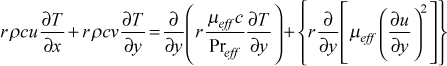 bl temp eqn
we see there is only one term in S_φ. This term is known as the viscous dissipation term, and it naturally arises from splitting the stagnation enthalpy equation by removing the reversible part of the viscous work (this is explained in detail in our textbook, CHMT). For accurate heat transfer calculations where either high Mach number effects or large temperature differences or large Prandtl number effects are expected, a variable property solution is required, and the stagnation enthalpy equation will automatically be solved.

The choices for jsor(j) for the energy equation are

jsor(j)	source terms - energy equation (stagnation enthalpy or temperature)
= 1	no energy equation source computed
= 2	add work term associated with X = ρg (gravitational body force, x-direction)
= 3	add (uτ) work term (viscous shear work, kfluid>1 or dissipation, kfluid=1)
= 5	add S (generalized energy source)
= 6	source is sum of flag =2 + flag =5
= 7	source is sum of flag =3 + flag =5
= 8	source is sum of flag =2 + flag =3 + flag =5

The following examples set up the flag kbfor and the flag jsor(j) array for various problem scenarios.

example: solve typical heat transfer problem - momentum and energy equations (neq=2)

momentum equation: dP/dx
energy equation (no viscous work - low-speed gas or low to moderate Pr liquid)

kbfor	jsor(1)	jsor(2)	jsor(3)	jsor(4)	jsor(5)
= 1	= 1

example: solve free convection problem - momentum and energy equations (neq=2)

momentum equation: dp/dx + rho*g (gravitational body force, x-direction) and note: g set using gxx
energy equation (neglect body force work, not important for most free convection problems)

kbfor	jsor(1)	jsor(2)	jsor(3)	jsor(4)	jsor(5)
= 2	= 1

example: solve typical heat transfer problem - momentum and energy equations - two-equation turbulence model (neq=4)

momentum equation: dP/dx
energy equation (viscous work - high-speed gas or low-speed high-Pr liquid)
turbulence kinetic energy equation
turbulence dissipation equation

kbfor	jsor(1)	jsor(2)	jsor(3)	jsor(4)	jsor(5)
= 1	= 3	= 11	= 21

Some final notes: the jsor(j)) entries can be left blank if neq=1 and only the momentum equation is being solved. They can also be left blank wherever they are not needed (see examples above). Traditionally the energy equation is j=1, but the internal logic for TEXSTAN generally permits any order for the various diffusion equations, except with kstart=0,10 where the order must be temperature, (followed by k and then ε if the flow is turbulent and a two-equation model is being used).

K top of page

k1

k1	flag definition
= 0	flag not used
= 1	virtual origin control (for kgeom=1,2,3 and kstart=3,4), virtual origin x_vo = gxx

The flag k1 allows the user to control the virtual origin to offset the variable xstart in the definition of the x-Reynolds number for external flows
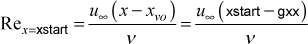
where the virtual origin x_vo is the input variable gxx. The issue of using a virtual origin is mostly important for auto-generating an initial turbulent velocity profile (kstart=3) when the user wants to start the computations at a given momentum thickness Reynolds number at the location x = xstart rather than at a given x-Reynolds number.

The laminar Blasius profile and the two-dimensional stagnation point region profile (for the cylinder in crossflow and for the turbine blade) are members of the Falkner-Skan flow family, and these profiles are created by specifying an x-Reynolds number, for which there will always be a unique momentum thickness Reynolds number. For the Blasius profile (m=0) and for the stagnation point profile (m=1) the virtual origin is identically zero.

The turbulent boundary layer velocity profile is developed by specifying the input-calculated x-Reynolds number to compute a turbulent friction coefficient and then using it to evaluate a turbulent power-law solution to create the velocity profile. This will produce a unique momentum thickness Reynolds number because of the correlation
that is only valid for moderate Reynolds number flows on smooth surfaces with zero pressure gradient.

If the user wishes have a different starting momentum thickness Reynolds number for a specified starting value of x, then the virtual origin concept will have to be used. We replace x by (x - x_vo) so that we can independently specify the x location and offset it with a virtual origin value x_vo. The value of the x-Reynolds number changes for a given x=xstart, and thus the starting momentum thickness Reynolds number changes, as can be seen in the turbulent friction factor equation. This is the primary idea behind using a virtual origin.

The adjustment is somewhat of an iterative process. To expedite the process, TEXSTAN prints the values of both Reynolds numbers at the first integration to the screen. The user can then quickly iteratively change gxx value by temporarily setting the flag k6 to some small number (say =3). This will cause TEXSTAN to terminate after 3 integration steps, and the user can input a new gxx value, until the required momentum Reynolds number for the initial profiles is generated. Obviously this iteration is not needed if there is no pressure gradient, because the above friction coefficient equality is exact. Otherwise, this is only approximate, but the procedure works.

k2

k2	value	flag definition
= 0		flag not used
= 1	Pr^1/2	recovery factor for laminar variable property external flows (mode=1 and kfluid>1)
= 1	Pr^1/3	recovery factor for turbulent variable property external flows (mode=2 and kfluid>1)
= 3	0.892	recovery factor for turbulent variable property external flows (mode=2 and kfluid>1)

The flag k2 is discussed in detail in the external flows: heat transfer section of this website. It is NOT designed for use with constant property calculations because of the ambiguity in how to interpret the free steam temperature in the energy equation that is technically programmed as a stagnation enthalpy equation.

For variable property flows, by use of the flag k2 the definition of the heat transfer coefficient can be easily switched from being based on the stagnation temperature, (T_s - T_∞*) to the adiabatic wall temperature (or recovery temperature), (T_s - T_aw).

k3: The flag k3 controls the print interval in all diagnostics files that are printed by use of the diagnostics flag k8 by printing at k3 multiples of the integration step counter, intg. The flag is very similar in function to kspace.

k4

The flag k4 permits the user to apply an analytical free stream velocity distribution, u_∞(x), for benchmark datasets that test the two-dimensional stagnation point flow and the cylinder-in-crossflow. Analytical distributions are convenient and provide very accurate pressure gradients, but use of the ubE(m) array is just as good, providing there are enough data points (nxbc on the order of 20 or more) and the data are shown to be smooth.

k4	flag definition
= 0	flag not used
= 5	u_∞(x) for Falkner-Skan m=1 2-D stagnation point flow (kgeom=1 and kstart=5)
= 6	u_∞(x) for cylinder-in-crossflow (kgeom=1 and kstart=6)

The commonly used laminar flows to test laminar boundary layer simulation codes include the flat plate flow described by the Falkner-Skan flow family (sometimes called wedge flows) and the cylinder-in-crossflow. These flows primarily test the pressure gradient effect on the laminar boundary layer. The initial conditions for these three flows are programmed into TEXSTAN (kstart=4 for Blasius, kstart=5 for Falkner-Skan, and kstart=6 for the cylinder). Currently TEXSTAN only has an analytical solution for m=1 when you choose kstart=5. Technically the cylinder-in-crossflow starting solution is the same as the m=1 starting solution, but we define it using kstart=6.

A Falkner-Skan flow is an external flow with a pressure gradient in which the free stream velocity u_∞ (x) is proportional to x^m Falkner-Skan uinf(x)
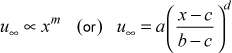
where a is the approach velocity, b is a distance scaling factor, c serves as a virtual origin, and d is the Falkner-Skan variable m. The TEXSTAN input variables for a, b, c, d are axx, bxx, cxx, dxx.

To test the two-dimensional stagnation point solution it is important to remember that TEXSTAN can not start at a x-Reynolds number of zero, but must start at a finite value. We can choose an arbitrary x-Reynolds number, for example =1000, and also choose the x location where Re_x=1000 will occur. This location will become the input variable xstart, and from the definition of the Reynolds number, the corresponding value for u_∞ at x=xstart at that location can be calculated. The other input variables will include b=bxx=1.0 for the distance scaling factor; c=cxx=0.0 for the virtual origin; d=dxx=1.0 for the Falkner-Skan m parameter. Based on these variable values the a=axx (the approach velocity) is uniquely determined. Note that if you choose axx (the approach velocity) then the solution for xstart will become iterative to satisfy the chosen value for Re_x and the m=1 free stream velocity distribution.

A cylinder-in-crossflow is an external flow with a pressure gradient in which the potential flow analytical free stream velocity u_∞ (x) is a sine function
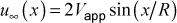
where the approach velocity V_app and the cylinder radius R are the input variables axx and bxx. Again, we can not start TEXSTAN at the stagnation point. As with the two-dimensional stagnation point flow, we can choose an arbitrary x-Reynolds number to start the computations, then evaluate the potential flow solution to determine what that value of u_∞ will be, and this will uniquely determine the value for xstart.

k5

The flag k5 serves two purposes. The first purpose is to cause a number of files to be written in addition to the standard output files. We call these files plotting files, but in reality they are just alphanumeric data containing arrays that can be easily imported into a plot package. The files have ftn in their name. There are a fixed number of ftn files for external and internal flows, and they mostly contain heat transfer coefficients, Nusselt numbers, Stanton numbers, friction factors, and other quantities. A review of these ftn files can be found in the overview: setup and run TEXSTAN section of this website.

The second purpose is to set the interval of print to these files, and it functions similarly to what kspace does in printing output to the file out.txt. By being able to specify both kspace and k5, the user can make the file out.txt small, while controlling the density of data points in the ftn for plotting (typically 500-1000 lines of data) for files that will rarely be physically printed.

k6: The flag k6 was designed to cause TEXSTAN to close all open print files and STOP when the integration counter intg reaches the value k6.

k7: The flag k7 is not currently used in academic TEXSTAN.

k8

The flag k8 has been designed to permit either printing of extra information or printing of diagnostic information to various ftn type files and often to the interactive DOS screen. The flag k3 controls the print interval of some of the ftn diagnostics files to be at k3 multiples of the integration step counter, intg. The overview: diagnostics section of this website gives an introduction to using flag k8. A summary of the print options include

k8	flag definition
= 0	flag not used
= 8	include the print of a self-explanatory array sp(5) in the file out.txt
= 9	cause a STOP to occur in TEXSTAN immediately after the input file is read and written to file in.txt
= 33	print finite-difference coefficients at intg = k3 to files ftn33.txt and ftn95.txt
= 34	print special k-ε diagnostics (useful only when installing a new model) to file ftn34.txt, and to files ftn73.txt and ftn74.txt
= 35	print diagnostics from subroutines that create auto-generated starting profiles to the interactive DOS screen, to file ftn35.txt and to files ftn73.txt and ftn74.txt
= 36	print analysis of boundary conditions as described in the overview: bc smoothness section of this website and then cause a STOP to occur in TEXSTAN
= 41	print free stream velocity and integration stepsize diagnostics (external flows) to file ftn41.txt at intervals of k3
= 42	print integration stepsize and entrainment diagnostics (external flows) to file ftn42.txt at intervals of k3
= 43	print pressure gradient and acceleration parameter diagnostics (external flows) to file ftn43.txt at intervals of k3
= 44	print entrainment diagnostics (external flows) to files ftn61.txt, ftn62.txt, and ftn63.txt at intervals of k3
= 46	print pressure gradient and iteration diagnostics (internal flows) to file ftn46.txt at intervals of k3
= 47	print model diagnostics (internal and external flows) to file ftn47.txt at intervals of k3

k9

k9	flag definition
= 0	flag not used
= 4	roughness model for use with the mixing-length turbulence model
> 0	momentum Reynolds number correlation for start of transition (Abu-Ghannam and Shaw, ktmtr=3 and Mayle, ktmtr=5) is replaced by input variable gxx, see modeling: transition

The flag k9 turns on the roughness model for use with the mixing-length turbulence model. The details of the model are described in detail in the modeling: roughness section of this website. Roughness effects in academic TEXSTAN are limited to the mixing length model and the one-equation model which uses the mixing length. The model is formulated as developed our textbook CHMT, and it is valid only for Nikuradse uniformly distributed roughness, characterized by the roughness length scale k_s and the roughness Reynolds number, Re_k = (k_s u_τ)/ν. The roughness length scale k_s is an input variable using cxx (units of m, SI, (or) ft, US/Eng) . Note, for kgeom=6,7, where there are two walls, and the input variable gxx (units of m, SI, (or) ft, US/Eng) is used to specify the roughness length scale for the E-surface (second wall).

k10

k10	flag definition
= 0	flag not used
= 10	nondimensional profiles at each x(m) for certain benchmark datasets and kout=8
= 11	dimensional profiles at each x(m) for kout=2,4
= 21	one set of dimensional profiles for external flows (kgeom=1,2,3) at a specified x-Reynolds number using variable bxx
= 22	one set of dimensional profiles for external flows (kgeom=1,2,3) at a specified momentum thickness Reynolds number using variable bxx
= 23	one set of dimensional profiles for external flows (kgeom=1,2,3) at a specified enthalpy thickness Reynolds number using variable bxx
= 24	one set of dimensional profiles for internal flows (kgeom=4,5,6,7) at a specified x/D_h using variable bxx
= 25	one set of dimensional profiles for any geometry at a given integration step intg using variable bxx

The flag k10 controls printing of profiles to the output file out.txt. There are two methods for choose the locations of the profiles that will be printed.

The first method is to set k10=10,11 and profiles will be printed at each x(m) location. With this method the user can easily add more x(m) points for profiles, and the drawback to this method is that it is based on the x location.

The second method is to set k10=21,22,23,24,25 and one set of profiles will be printed, but the location is more precise. The input variable is bxx.

More details of the printing can be found in the internal flows: output files and external flows: output files sections of this website.

k11: The flag k11 is not currently used in academic TEXSTAN.

k12

This flag is no longer used and it is set =0.

The flag is mostly a carryover from the boundary layer code STAN5, the predecessor to TEXSTAN. In former times (the 1950s and 1960s), when computer core and execution speed were a premium, external boundary layer solutions for aerodynamic design had to be carried out using integral methods. By the mid 1960s a hybrid scheme was adopted that incorporated both an integral method (or the famous law-of-the-wall algebraic equation substitute) and a differential method. By the 1970s a complete differential method was possible. In the early years of the STAN5 it could function as a hybrid scheme, and TEXSTAN is truly a differential method. The transition from hybrid to pure differential meant that five to ten times (or more) finite difference points were needed for the cross-stream direction. This was especially important for external turbulent flows, where the requirement for several finite difference points within the laminar sublayer was needed for maintaining numerical accuracy. For numerical formulations in codes such as STAN5 and TEXSTAN, where the grid was continually expanding (for external flows only), it was possible to eventually violate the requirement for the number of points within the sublayer region of turbulent flow. Therefore an algorithm was incorporated to continually test the second finite-difference point away from a surface and if it became too large and violated the requirement y⁺ ≤ 0.2, a new finite difference point was added near the surface. This maintained numerical accuracy, but at one time it also caused some stability problems, especially when a turbulent boundary layer was being subjected to an adverse pressure gradient (or blowing) that caused the boundary layer to enlarge rapidly. The k12 flag was adapted as a means to switch off the new-point addition algorithm when k12=1.

kbfor

The x-momentum equation requires the kbfor flag to define what type of momentum source to consider. The value of kbfor must be ≥1.

kbfor	x-momentum equation source terms
= 1	dp/dx (pressure gradient)
= 2	dp/dx + rho*g (gravitational body force, x-direction) and note: g set using gxx
= 3	dp/dx + X (generalized X body force per unit volume)
= 4	the combination of options 1 + 2 + 3
= 5	dp/dx + flow-direction curvature (mixing-length and 1-equation turbulence models)

If kbfor=1, the momentum equation will compute only the pressure gradient (dp/dx) as a source term.

For external flows, the pressure gradient is formed from the Bernoulli equation by numerically differentiating the free stream velocity distribution using a first-order differencing scheme. Note the velocity distribution is obtained by cubic-spline interpolation. A Blasius boundary layer requires a constant free stream velocity, and thus dp/dx will be =0.0. This still requires kbfor=1.

For internal flows, at each integration step in the x-direction, the pressure gradient is unknown. Therefore, to solve the momentum equation, the dp/dx is guessed, the momentum equation solved, and the u-velocity*density profile is integrated between the I- and E-surface to determine the mass flow rate per unit span. This flow rate is compared to the initial mass flow rate as computed from the initial conditions, and dp/dx is iterated until the solution converges. Integration then proceeds to the next x location. Note that on rare occasions, this procedure fails to converge and TEXSTAN abruptly stops.

If kbfor=2, a rhoc*gv body force per unit volume due to free or mixed convection is added to the pressure gradient. The value of g is supplied by the input variable gxx. Its sign convention is plus if the direction of action of g is in the +x flow direction and minus if the direction of action of g is in the -x direction. For example, flow on a heated vertical flat plate would be upward, and the direction of the gravitational force is in the opposite direction; g = -9.8 m/s^2 or -32.17 ft/s^2; aided mixed convection would be forced convection in the same direction as the gravitational force, requiring g to be a positive value; opposed mixed convection would have the forced flow moving upward against the direction of g.

Note that internal flow mixed convection is overall iterative. The inlet and exit pressures of the internal flow channel are known but not the mass flow rate. The user has to guess the input velocity (a flat profile) to establish a mass flow rate, and then iterate the TEXSTAN solution until the overall channel pressure drop matches the physical problem. Note further that some mixed convective flows result in a reverse flow at the exit. This is not a possible solution in TEXSTAN.

if kbfor=3, a generalized body force per unit volume, X, is added to the pressure gradient. This generalized body force is input by the aux3(m) array and linearly interpolated. An example might be a magnetohydrodynamic body force.

If kbfor=4, the pressure gradient is combined with the free/mixed convection body force and the generalized body force.

If kbfor=5, the effect of surface longitudinal curvature is added to mixing length turbulence models for boundary layer flow (kgeom=1 and ktmu=1-5, or with ktmu=11). In addition, the pressure gradient is calculated for the momentum equation. The radius of curvature of the surface is input by the aux3(m) array. Note that curvature terms are not programmed into the governing equations.

kdx

kdx	flag to control how integration stepsize is computed
= 0	compute using the variable deltax
= 1	compute by interpolation of the input array aux1(m)

kent

The variable kent is applicable only to external flows, and for internal flows, kent must be set =0, even though it is not used, because of the way the TEXSTAN's input file read structure is designed.

kent	entrainment model
= 0	base entrainment on velocity profile only
= 1	base entrainment on all dependent variable profiles
= 2	base entrainment on velocity and temperature (or stagnation enthalpy) profiles
= 3	base entrainment on all profiles except dissipation profile

For fluids with a Prandtl number is < 1 and considering heat transfer, the thermal boundary layer will be larger than the velocity boundary layer. Choosing kent=0 (entrainment based only on the velocity boundary layer) will result in numerical accuracy problems.

More information can be found in fra and enfra, and a general discussion of entrainment can be found in the external flows: integration control section of this website.

kfluid

kfluid	fluid properties
= 1	all fluid properties are held constant
> 1	fluid properties are variable

kfluid	variable property fluid model
= 2	air at low pressure (adapted from our textbook CHMT)
= 4	water
= 6	nitrogen
= 8	helium
= 14	air ideal gas, Pr=const, c_p=const, Sutherland viscosity law
= 15	air similar to kfluid=14 but sets (ρ*μ)=const
= 16	motor oil (adapted from our textbook CHMT)

The properties in TEXSTAN can be considered constant or variable. Solution to the energy equation is mandatory for variable properties. A decision to use variable properties is generally based on the ratio of the expected wall to mean absolute temperature (or free stream temperature). When this ratio falls outside the interval from 0.95 to 1.05, the user should test the solution by recomputing the solution using variable properties to insure the constant property assumption does not substantially affect the results. Note that use of variable properties does not require consideration of viscous work (or the effect of viscous dissipation). This is an independent effect.

The details of each model can be found in the overview: fluid properties section of this website.

kgeom

kgeom	geometry for external boundary layer flows
= 1	boundary layer flow on a 2-D planar surface (flat plates, 2-D airfoils, 2-D "flat" nozzles)
= 2	boundary layer flow over an axisymmetric body of revolution (missiles, spheres)
= 3	boundary layer flow inside an axisymmetric body of revolution (axisymmetric nozzles)

kgeom	geometry for internal flows
= 4	flow in a circular pipe
= 5	flow between parallel planes or in flat ducts (requires symmetric thermal boundary conditions)
= 6	flow between parallel planes or in flat ducts (symmetrical or asymmetric thermal boundary conditions)
= 7	flow in an annular duct

The external flow class requires specification of dp/dx in the flow direction via the edge (free stream) velocity distribution. The effect of curvature in the direction of flow can be accounted for only for the specialized mixing length model (kbfor=5). Otherwise, flow-direction curvature terms are not programmed into the governing equations. Transverse curvature for axisymmetric flows is exactly accounted for by use of the axisymmetric form of the governing equations.

The kgeom=1 geometry is a planar geometry, and the geometry includes flow over flat plates, over airfoils, and inside high aspect ratio 2-D converging-diverging nozzles (either subsonic or supersonic isentropic). Computations are carried out from the wall (I-surface) to the free stream (E-surface). The planar flow is computed per unit width.

The kgeom=2 geometry is the axisymmetric flow over bodies of revolution, such as a missile. Computations are carried out from the wall (I-surface) to the free stream (E-surface). The axisymmetric flow is computed per unit radian.

The kgeom=3 geometry is the axisymmetric flow inside converging-diverging nozzles (either subsonic or supersonic isentropic). Computations are carried out from the wall (I-surface) to the free stream (E-surface). Note that the flow in the converging section remains a boundary layer type of flow only because the distance to the edge of the boundary layer is very small in relation to the distance from the wall to the axisymmetric centerline. This assumption will become marginal for the diverging section as the flow entrains fluid in an attempt to remain an attached flow. The axisymmetric flow is computed per unit radian.

The internal flow class does not require specification of dp/dx in the flow direction. In fact, it is an unknown and thus requires iteration at each x-step to satisfy conservation of mass.

The kgeom=4 geometry is the axisymmetric flow in a circular pipe. Computations are carried out from the symmetry line or centerline (I-surface) to the wall (E-surface). The flow is computed per unit radian.

The kgeom=5 geometry is the planar flow between parallel plates. This approximates flow in a flat, high aspect-ratio duct. The flow is computed per unit width. The kgeom=6 geometry is similar. Which to choose depends on the thermal boundary conditions. If they are symmetric, choose =5, and if they are different or asymmetric (i.e. one wall heated and one wall adiabatic), choose =6. The symmetric geometry computations are carried out from the centerline (I-surface) to the wall (E-surface). The asymmetric geometry computations are carried out from the lower wall (I-surface) to the upper wall (E-surface).

The kgeom=7 geometry is the annulus. The flow is computed per unit radian. The computations are carried out from the inner wall radius (I-surface) to the outer wall radius (E-surface).

kloc

kloc	flag definition
= 0	flag used with kstart=0,10 to tell TEXSTAN the user-supplied initial profiles (or restart profiles) are within the input data set
= 1	flag used with kstart=0,10 to tell TEXSTAN the user-supplied initial profiles (or restart profiles) are located in a separate initial profiles data set

The flag kloc is only used for user-supplied initial profiles. The operational use of this variable is described in the external flows: initial profiles section of this website.

kout

kout	output file format for file out.txt
= 2	external (boundary layer) flow format (kgeom=1,2,3)
= 4	internal (pipe and channel) flow format (kgeom=4,5,6,7)
= 6	generalized format for all kgeom
= 8	specialized format for benchmark datasets
= 9	specialized output for transitional flows (ktmtr>1 and kgeom=1)

Standard output goes to the output file out.txt. All output has a brief list of input variables at the top, followed by a set of output data that are printed at integration intervals set by the input variable kspace.

The standard external flow output file (kout=2) includes the x-Reynolds number (Re_x), momentum thickness Reynolds number (Re_m), friction coefficient (c_f /2), shape factor (H₁₂), enthalpy thickness Reynolds number (Re_h), and Stanton number (St).

The standard internal flow output file (kout=4) includes the ratio of flow distance to hydraulic diameter (x/D_h), apparent friction coefficient (c_f,app), surface friction coefficient (c_f /2), and, Nusselt number (Nu).

file	geometry	variables
out.txt for kout=2	(kgeom=1,2,3) External Flows	Re_x , Re_m , c_f /2 , H₁₂ , Re_h , St
out.txt for kout=4	(kgeom=4,5,6,7) Internal Flows	x/D_h , c_f,app , c_f /2 (I), c_f /2 (E), Nu(I), Nu(E)

A more complete discussion of output for external flows can be found in external flows: output files section of this website, and a more complete discussion of output for internal flows can be found in internal flows: output files section of this website.

Option kout=6 is rarely used today. It produces a large amount of raw data and was developed primarily as a diagnostic tool for code development. Most of the data content from this option can be printed to files using other output choices controlled by the k-flags.

Option kout=8 has been constructed primarily to test benchmark data sets that are supplied with TEXSTAN. As such, this option compares nondimensional numbers with standard convective heat transfer correlations, built into the output subroutine and mostly adapted from our textbook CHMT. The use of benchmark data sets is crucial to understanding how data sets are constructed, and it provides an easy check of whether the TEXSTAN data output is following the expected theory.

Option kout=9 was developed to track the evolution of transitional boundary layers as they progress from laminar flow to turbulent flow. The output routine has logic which generally works, but sometime fails to completely track the changeover. This output routine can be used both with flat plate flows (kstart=4) and turbine blade flows (kstart=7).

kspace

The flag kspace controls the print interval in output file out.txt by printing at kspace multiples of the integration step counter, intg. In addition there will always be a print at intg=5 and at the final intg value. For example, if kspace=100, there will be print at intg=5, intg=100, intg=200, intg=300, and so forth, followed by a print at the last intg location.

Note there is an upper limit to the number of integration steps that TEXSTAN will allow (currently 30,000).

kstart

kstart	external flow initial profiles
= 3	turbulent velocity and temperature profiles for kgeom=1,2,3; includes k and ε profiles
= 4	Blasius velocity and temperature profiles for kgeom=1
= 5	Falkner-Skan m=1 (2-D stagnation point) velocity and temperature profiles for kgeom=1
= 6	cylinder-in-crossflow velocity and temperature profiles for kgeom=1
= 7	turbine blade velocity and temperature profiles for kgeom=1;
= 9	flat profiles of all variables for kgeom=1 (used on highly rough surfaces)

kstart	internal flow initial profiles
= 1	flat entry profiles of velocity and temperature for kgeom=4,5,6,7; note: includes k and ε profiles
= 2	laminar hydrodynamically fully-developed velocity profile with either a flat or thermally fully-developed temperature profile for kgeom=4,5,6,7
= 3	turbulent velocity and temperature profiles for kgeom=4,5,6; includes k and ε profiles
= 11	Couette flow velocity and temperature profiles for kgeom=6, laminar or turbulent flow

kstart	special user-supplied initial profile options
= 0	primarily designed for restart of TEXSTAN based on a dump of profiles from a previous calculation
= 10	primarily designed to input experimental profiles, selected kgeom and turbulence models

The TEXSTAN-generated external flow initial profiles for laminar flow are restricted to the Blasius flow and the accelerated Falkner-Skan m=1 flow and kgeom=1. The Falkner-Skan m=1 profile is the 2-D stagnation profile in which the free stream velocity linearly accelerates, and thus it can be applied as a first approximation to the cylinder in crossflow and to the cylindrical leading-edge region of a turbine blade (airfoil). For turbulent flows and kgeom=1,2,3, classical power-law profiles are used as an approximation. All temperature profiles will be constructed as stagnation enthalpy profiles if variable properties are being considered.

The TEXSTAN-generated internal flow initial profiles for laminar flow are designed for one of three flow cases: (a) the combined entry flow where the velocity and temperature profiles are flat; (b) the unheated starting length flow where the velocity profile is hydrodynamically fully-developed and the temperature profile is flat; and (c) the thermally fully-developed flow. For turbulent flow the choices are either combined entry flow or thermally fully-developed flow where the profiles are approximated by the classic power-law profiles. For higher order turbulence models the entry flow profile choice is best. All temperature profiles will be constructed as stagnation enthalpy profiles if variable properties are being considered.

The kstart=1 option for kgeom=4,5,6,7 generates flat profiles for all dependent variables. Note that if the energy equation is being solved, a temperature profile is created, and it is converted to a stagnation enthalpy profile only if variable properties are being considered.

The kstart=2 option has limited options for kgeom=4,5,6,7. It is primarily intended to generate fully-developed laminar velocity profiles coupled with a flat temperature profile to begin an unheated starting length problem for all four kgeom values. For kgeom=4, a fully-developed temperature profile can also be generated for both a constant wall temperature and constant wall heat flux boundary condition. For kgeom=5, a fully-developed temperature profile can also be generated for a constant wall heat flux boundary condition. For kgeom=6 a fully-developed temperature profile can also be generated for a constant wall heat flux boundary condition, provided the thermal boundary conditions are symmetrical.

The kstart=3 option for kgeom=1 or for kgeom=4,5,6 generates turbulent velocity and temperature profiles by solving the Couette flow equation for the near-wall region and matching them to power-law profiles for the outer region. Mixing length and a constant turbulent Prandtl number are used for the turbulence model. If k and ε profiles are required, they are calculated for the near-wall region based on the theory for TEXSTAN's one-equation k-model. For the outer region, the k and ε profiles are matched in value and derivative using a 3rd order polynomial, insuring continuity of the k and ε profiles.

The kstart=4,5,6,7 options are used to generate various laminar boundary layer profiles for kgeom=1,2,3. For kstart=4 Blasius boundary layer profiles are created; for kstart=5,6,7 the 2-D stagnation point flow profiles are created, corresponding to the m=1 Falkner-Skan solution. For these kstart values, the Falkner-Skan equations are integrated in subroutine prof using a Runge-Kutta scheme. This is not a shooting method, in that the appropriate derivatives are supplied via curve fits. The reference for the solution scheme is found in White (1974).

The Falkner-Skan solution is valid for 0.6≤ Pr≤ 15; 0.99 ≤ (twall/tinf) ≤ 1.01; Mach number ≤0.05; constant or variable properties; constant wall temperature boundary conditions. The user can violate these criteria, and although the initial profiles will not be correct, TEXSTAN will eventually adjust. Note that for kstart=5,6 TEXSTAN has an option using the k4 input variable to provide a theoretical free stream velocity distribution.

The kstart=9 generates flat profiles for velocity and temperature. This option requires specification of a common boundary layer thickness using the input variable gxx, and requires the energy equation to be solved. Note, this =9 option is rarely needed, except for some rough-surface flows.

If turbulence kinetic energy (k) and turbulence dissipation (e) profiles are required for a transitional boundary layer calculation and kgeom=1,2,3 the k profile is scaled as a quadratic function of the laminar velocity profile and the e profile is 0.3*k*du/dy. Beyond the peak in k and peak in ε for the near-wall region, the ε profile is matched in value and derivative using a 3rd order polynomial and smoothly connected to its free stream value.

If a mass transfer concentration (m_j) profile is required for kgeom=1, it is scaled from the non-dimensional velocity profile, with the y-location for the scaled m_j profile itself scaled using Schmidt number to the 1/3 power.

The kstart=0 option really should only be used to restart TEXSTAN when the profiles come from a previous run of TEXSTAN. For example, the user could cause TEXSTAN to print dependent variable profiles using the k10 flag at a particular location. These profiles could then be incorporated into a new data set. This is particularly useful for the study of turbulence models. A second example is to generate k-e profiles that are compatible with the k-e equations. TEXSTAN can be started at a low x-Reynolds number, allowed to go through transition, and then print all profiles using k10=22 at a low turbulent momentum Reynolds number. The resulting file can then be used with kstart=0.

Note that TEXSTAN uses the initial velocity profile distribution to establish the finite difference grid, and thus the distribution is quite important to obtaining a grid-independent (as well as stepsize independent) solution. Use of kstart=0 can often lead to solutions that are not grid independent, unless the user follows the procedure described in the previous paragraph to create a set of profiles, especially for turbulent flow.

The kstart=10 option is useful if the user plans to start TEXSTAN with experimental profiles. The profiles are read and then interpolated onto a grid using the user-specified mesh variables dyi and rate. If the energy equation is being solved, it is assumed the user has supplied an initial temperature profile. If variable properties are being considered, the temperature profile is converted to a stagnation enthalpy profile. If the user is considering an experimental turbulence kinetic energy profile but not the corresponding experimental dissipation profile, and intends to use a two-equation turbulence model, TEXSTAN has the provision to create a turbulence dissipation profile. This choice is flagged using the epsapp variable.

ktme

ktme	turbulence model for the energy equation (heat transfer)
= 0	for all flows that start laminar and remain laminar
> 0	for all flows that start laminar and are permitted to transition, or for flows that start turbulent

ktme	turbulence model for the energy equation
= 1	constant turbulent Prandtl number; =0.90
= 2	constant turbulent Prandtl number, = fxx
= 3	Kays variable turbulent Prandtl number model

The TEXSTAN model for turbulent heat flux (or eddy diffusivity for heat) is based on the turbulent Prandtl number, which is used in conjunction with the turbulent viscosity (or eddy diffusivity for momentum) to obtain the turbulent conductivity. There are two model choices in TEXSTAN: a constant turbulent Prandtl number or a turbulent Prandtl number that varies in the cross stream direction. The models are described in detail in the modeling: turbulent Prandtl number section of this website.

Although the variable turbulent Prandtl number model was derived to work with the mixing-length turbulence model, it works equally well for fully turbulent flows with 1- and 2-equation turbulence models, but it is not recommended for transitional boundary layer flows or flows with pressure gradients. For turbulent mass transfer, the turbulent mass flux would be specified through a turbulent Schmidt number. However, there is currently no provision in TEXSTAN to input a turbulent Schmidt number.

ktmtr

ktmtr	transition model for the momentum equation
= 0	for all flows that start laminar and remain laminar
> 0	for all flows where transition is permitted

ktmtr	transition models for boundary layer flows (turbulence intensity Tu > 2-3%)
= 1	abrupt mixing-length transition (requires mode=1 and gxx)
= 2	used for the ktmu=23 k-ε turbulence model (requires mode=2 and axx)
= 3	Abu-Ghannam/Shah mixing-length transition (requires mode=1)
= 4	Kays/Crawford mixing-length transition (requires mode=1)
= 5	Mayle mixing-length transition (requires mode=1)

Transitional external flows in TEXSTAN can be modeled using any of the three classes of turbulence models: mixing length, one-equation k, and two-equation k-ε. The transition models are described in detail in the modeling: transition section of this website.

For mixing-length or one-equation turbulence models the transition model can be either a distributed model or an abrupt model. The distributed model is typically associated with bypass transition and is applicable to free stream turbulence (Tu) values that are greater than 2-3%. Bypass transition is a process where the traditional transition flow structures are not seen as the flow moves from disturbed laminar flow to fully turbulent flow. It can be characterized by two Reynolds numbers that describe the start location where the friction will be expected to be about 10% larger than its laminar value at the same Reynolds number, and the end location where the friction will be within about 90% of its turbulent value for the same Reynolds number. With the abrupt model, the flow begins in a laminar state, and when the flow exceeds some criteria such as a critical Reynolds number the turbulent viscosity is computed and added to the laminar viscosity. This model is often applied to flow over rough surfaces or when there is an identifiable boundary layer trip.

For the two-equation turbulence transition model, TEXSTAN computations are started at a very small x Reynolds number, and the k-ε equations are computed along with the x-momentum equation. The turbulent viscosity is added to the laminar viscosity from the start of computations, and as the k-ε profiles begin to develop, the turbulent viscosity becomes significant, causing the friction and heat transfer to move from a laminar value and approach a turbulent value. This type of transition has been called a natural two-equation transition. Typically this results in early transition, and the transition length (from the point where the friction is 10% greater than its laminar value to the point where it is within 90% of its fully turbulent value) is too short. To change this, the k-equation is modified to control the production of (k). It works fairly well for turbine blade transition, but needs further adjustments.

For very low Tu values, (< 2-3%) such as on compressor blades, some low-Re turbine blades, reentry vehicles, and flight vehicles at high altitude, the transition modeling needs to be very precise, and this type of transition is not addressed in TEXSTAN.

ktmu

ktmu	turbulence model for the momentum equation
= 0	for all flows that start laminar and remain laminar
> 0	for all flows that start laminar and are permitted to transition, or for flows that start turbulent

ktmu	mixing-length model choices for external boundary layer flows
= 1
= 2
= 3
= 4
= 5

ktmu	mixing-length model choices for internal flows
= 6
= 7
= 8

ktmu	one-equation turbulence kinetic energy model choice for external flows
= 11	Hassid-Poreh

ktmu	two-equation turbulence kinetic energy-energy dissipation model choices for internal and external flows
= 21	Launder-Sharma
= 22	KY Chien
= 23	Lam-Bremhorst
= 24	Jones-Launder

Models for the turbulent viscosity (or eddy diffusivity for momentum) include the mixing length model, the one-equation k model, and the two-equation k-ε model. The flag ktmu identifies the model for computing the turbulent viscosity. Some of the models contain input variables axx, bxx, cxx, dxx, exx to allow the user to change the built-in turbulence model values.

The TEXSTAN code has a choice of numerous mixing length models for both internal and external flows. These models are described in detail in modeling: mixing length model section of this website. For external flows the mixing-length model incorporates the van Driest damping function, with the A⁺ model being a function of both pressure gradient and transpiration and damped by a first-order lag equation. Models for roughness and curvature can be used in conjunction with the external-flow mixing-length.

For internal flows there is a choice of either a pure mixing-length model or a hybrid mixing-length and constant eddy diffusivity model. The mixing-length model incorporates the van Driest damping function, with the A⁺ being a constant value. For the hybrid model a constant eddy diffusivity for momentum is computed as a function of hydraulic diameter Reynolds number for the outer layer away from a wall. The outer layer model is used when its value exceeds the mixing-length model value or when the distance from the wall exceeds a certain value. This hybrid model is valid only for fully-developed pipe flow and fully-developed flow between parallel planes. A model for surface roughness can also be used in conjunction with the mixing-length model.

For external flows the one-equation turbulence-kinetic-energy can be used in conjunction with the mixing-length model for the required length scale. This model is described in detail in the modeling: one-equation model section of this website. Because the one-equation model uses the mixing length, it has also been adapted to the curvature model. A primary advantage of the one-equation model is that it can incorporate the effects of the free-stream turbulence via the outer boundary condition for the k-equation.

For both internal and external flows, the TEXSTAN code has a choice of four two-equation k-ε turbulence models. These models are described in detail in the modeling: two-equation model section of this website.

kunits

kunits	units for all dimensional input variables to TEXSTAN
= 0	U.S. Customary (British or English) units system
= 1	SI (metric) units system

TEXSTAN works in dimensional variables that must adhere to either the U.S. Customary Units convention (often called the British or English unit system) or the SI units convention (often called the metric unit system). To permit this flexibility, the force-mass conversion factor from Newton's Second Law, g_c , and the work energy-heat energy conversion factor, J , are programmed into the equations as the FORTRAN variables gc and cj. The details of these two units systems can be found in the overview: units section of this website.

L top of page

M top of page

mode

mode	flag to set the initial state of flow: laminar or turbulent
= 1	turbulent transport terms are not calculated
= 2	turbulent transport terms are calculated

The flag setting mode=1 is required for laminar internal flows and laminar boundary layer flows that are not permitted to become turbulent.

The flag setting mode=2 is required for turbulent internal flows and turbulent boundary layer flows when the initial profiles are being calculated using the turbulent initial profile generator kstart=3 or when the user is supplying experimental turbulent initial profiles kstart=10.

The flag setting mode=2 is required for any flow that uses a two-equation turbulence model. This includes entry region of turbulent channel flows and the laminar region of transitional boundary layers. The turbulent transport terms will contribute to the simulation of transition through the entry region (internal flows) or the low-Reynolds number laminar region (external flows).

For transitional boundary layer flows using a mixing-length transition model, mode=1 is required, and switch over to turbulent flow (mode=2) will occur by way of the turbulence model.

N top of page

neq

The flag neq tells TEXSTAN how many transport equations it will solve.

neq	number of transport equations to be solved by TEXSTAN
= 1	solve only the momentum equation
> 1	solve momentum equation + (neq-1) diffusion equations

The minimum value is =1 and the maximum value is =6. For the minimum TEXSTAN only solves the momentum problem. Otherwise TEXSTAN solves the momentum equation and one or more diffusion transport equations for scalars. Examples of diffusion equations currently within TEXSTAN include:

stagnation enthalpy equation (variable properties)
temperature equation (constant properties)
turbulence kinetic energy (k) equation
turbulence dissipation (ε) equation
mass concentration of component A in and A-B boundary layer

In the strictest sense TEXSTAN is a parabolic partial differential equation solver for equations of a common form. The equations all have the boundary layer approximations applied to them (one-dimensional pressure and cross-stream gradients much greater than streamwise gradients). The formulation for TEXSTAN follows the original formulation by S. V. Patankar and D. B. Spalding (Heat and Mass Transfer in Boundary Layers, Morgan-Grampian, London, 1967) where they identified the momentum equation differently from all other equations, which were then labeled diffusion equations.

All of the diffusion equations have a common structure, shown here in axisymmetric coordinates (which is the form programmed into TEXSTAN)

where C equals unity for momentum, and for the various scalar transport equations (stagnation enthalpy, temperature, mass concentration, turbulent kinetic energy, turbulent dissipation) it represents the appropriate non-dimensional effective transport coefficient. The S_φ term represents the collective of all source and sink terms for the dependent variable in question. A complete discussion of this equation can be found in the generalized transport equation part of the overview: transport equations section of this website.

The upper limit to the number of diffusion equations is specified in two include files in its source code: abc.inc and size.inc, and it is currently set =5 by the parameter variable njeqns. TEXSTAN then uses the input variable neq to determine the upper limit of FORTRAN do-loops associated with boundary condition and other information for each diffusion equation. These variables can only be changed by recompilation of the code.

nxbc(E): See nxbc(I) - which contains both definitions.

nxbc(I)

The flag nxbc(I) tells TEXSTAN the number of boundary locations along the I-surface. TEXSTAN requires the same number of boundary conditions along the E-surface. Therefore nxbc(I) = nxbc(E). The physical flow domain that defines these surfaces is further described in the external flows: integration control and internal flows: integration control sections of this website.

Numerical values for nxbc(I) and nxbc(E) range from 2 (minimum) to 101 (maximum). The boundary condition values are mostly linearly interpolated between locations. Exceptions are as follows: free stream velocity is spline-interpolated; free stream turbulence variables are changed via their respective turbulence model; and the free stream stagnation enthalpy (or temperature, if constant properties) is constant.

O top of page

P–Q top of page

po

Fluid pressure (units are N/m², SI; lbf/ft², US/Eng)

po	definition
P_∞	initial static pressure (external flows, constant property gases)
P_∞^*	stagnation (total) pressure (external flows, variable property gases
P_inl	initial static pressure (internal flows, constant and variable property gases and liquids

Because of the boundary layer assumptions and the assumption of no effect of curvature on pressure, the fluid static pressure will be constant over the flow cross-section for both internal and external flows. It is assumed that po is the pressure at the location of the start of the calculations, x=xstart.

For external flows, if the input variable is interpreted as a stagnation or total pressure, it is immediately converted to a static pressure using the 1-dimensional perfect gas formulation ratio Ptotal/Pstatic
and γ is the ratio of specific heats. The γ variable is either an input variable gam/cp for the kfluid=14,15 perfect-gas model, iteratively calculated for kfluid=13, or it is an entry in variable property tables for the other gas model options.

For both constant and variable properties, the static pressure is changed during integration using the Bernoulli equation and the free stream velocity distribution, static P integral external flow

For internal flows, the pressure is changed during integration by first establishing the local pressure gradient at each x location using an iterative scheme to satisfy the axial flow direction conservation of mass at that location, and then integrating in a manner similar to how the external pressure gradient is integrated. static P integral internal flow

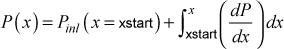
prc(j)

The variable prc(j) corresponds to the variable C_φ variable in the generalized transport equation for each diffusion equation. The logic for this array is very similar to that used for the jsor(j) array. The common structure of all the equations (see Generalized Transport Equation in the overview: transport equations section of this website) is reproduced here in the form programmed into TEXSTAN (axisymmetric coordinates) general conv-diff eqn
where C_φ equals unity for momentum, and for the various scalar transport equations it represents the appropriate non-dimensional effective transport coefficient. The C_φ term corresponds to the prc(j) variable. Examples of diffusion equations currently within TEXSTAN include:

i^* , stagnation enthalpy equation (variable properties,kfluid>1)
T , temperature equation (constant properties, kfluid=1)
k , turbulence kinetic energy equation
ε , turbulence dissipation equation
m_j , mass concentration of component A in and A-B boundary layer

and the corresponding prc(j) values will be

prc	type of diffusion transport equation
C_φ = Pr	energy equation (the Prandtl number)
C_φ = 1.0	turbulence kinetic energy equation model (required value)
C_φ = 1.0	turbulence dissipation equation model (required value)
C_φ = Sc	mass transfer equation (the Schmidt number)

For the energy equation, the following applies, depending on the properties choice

prc(j)	kfluid	Prandtl number
= (input variable)	= 1	Pr value supplied by user
= 0.0	= 2,4,6,8,16	TEXSTAN interpolates using table lookup
= 0.0	= 13	TEXSTAN computes from Pr(T) correlation
= (input variable)	= 14,15	Pr value supplied by user

For the mass transfer equation, only constant properties can be used.

warning There is a special circumstance if only the momentum equation is being solved, because neq=1 suggests there will be no prc(j) values required. However, the structure of TEXSTAN input is to read this data line for prc(j) because it is in the sequence of read statements and the structure of all input data sets for TEXSTAN is similar. Therefore, do NOT leave this data line out when neq=1. Keep the data line (and its dataline header) in the data sequence, and it will be read and then ignored, regardless of what values are entered for prc(1) and so forth.

R top of page

rate: The variables rate and dyi set the y spacing for the velocity profile, which in turn controls the grid (finite difference mesh) for TEXSTAN. These variables are explained in considerable detail in the external flows: initial profiles and internal flows: initial profiles sections of this website.

reyn: For internal flows this is the inlet hydraulic diameter Reynolds number, defined in the internal flows: Reynolds number section of this website.

rhoc

Fluid mass density (units are kg/m³, SI; lbm/ft³, US/Eng)

rhoc	kfluid	density
= (input variable)	= 1	ρ value supplied by user
= 0.0	= 2,4,6,8,16	TEXSTAN interpolates using table lookup
= 0.0	= 13,14,15	TEXSTAN computes from ideal gas law

rw(m)

Transverse curvature array that contributes to defining a given geometry (units are m, SI; ft, US/Eng).

rw(m)	kgeom	definition
= 1.0	=1	arbitrary value for external planar surfaces
= r_s(x)	= 2,3	wall radius of the I-surface for external axisymmetric surfaces
= r_s	= 4	pipe radius (may not vary with x)
= a	= 5	half-height distance (centerline-wall) for parallel-planes channel (height may not vary with x)
= 2a	= 6	full-height distance (wall-wall) for parallel-planes channel (height may not vary with x)
= r_i	= 7	inner-surface radius of annulus - aux2(m) sets outer-surface radius (gap may not vary with x)

For kgeom=1 (boundary layer on a planar surface), rw(m) is not important, but it must be set to some value and not left blank.

For kgeom=2,3 (axisymmetric boundary layer flows over a surface of revolution such as a sphere or missile or inside an axisymmetric nozzle) the I-surface is the wall and the E-surface is the free stream. The rw(m) array represents the transverse radius of curvature of the I-surface radius, as measured from the axis of revolution that generates that surface. This invariably presents a problem because typically the radius is only known with respect to distance along the axis of revolution (z). Thus the user must first determines the wall radius with respect to z and then map it into the intrinsic value with respect to x.

For kgeom=4 and kgeom=7 (circular pipe and annulus) the relationship between z and x is 1:1, and the rw(m) array represents the E-surface radius (for the pipe wall) and the I-surface radius (the inner wall for an annulus). For the annulus, the outer radius will be established by adding the contents of the aux2(m) array to the rw(m) array. In academic TEXSTAN pipe radius or annular cross-section is not allowed to vary with x to create a diffuser or nozzle geometry.

For kgeom=5 (thermally symmetric parallel planes duct) the rw(m) array represents the half height of the duct (distance between the I- and E-surfaces). In academic TEXSTAN the duct width is not allowed to vary with x to create a diffuser or nozzle geometry.

For kgeom=6 (full parallel planes duct) the rw(m) array represents the full height of the parallel planes (distance between the I- and E-surfaces). In academic TEXSTAN the duct width is not allowed to vary with x to create a diffuser or nozzle geometry.

S top of page

T top of page

title

This is a user-specified alphanumeric data line that will appear on all TEXSTAN output data files. The line can have between 1 and 80 characters, and it serves primarily to describe the data set. As an example, consider the title used in the benchmark data set s10.dat.txt for the Blasius boundary layer:

s10.dat lam bl, flat plate, t=const bc

The title describes part of the data set name (s10.dat), that it is a laminar boundary layer on a flat plate (lam bl, flat plate), and that the surface thermal boundary condition is a constant surface temperature (t=const bc)

tref: For internal flows this variable is the initial or inlet value of the mass-averaged temperature (or bulk temperature) of the fluid in units of ºC or K, SI (or) ºF or ºR, US/Eng at x = xstart. The mass-averaged temperature will only change in response to surface heat transfer. The use of this variable is presented in the internal flows: initial profiles section of this website. Note: if only the momentum equation is being solved, tref must be set =0 because of the way the TEXSTAN's input file read structure is designed.

tstag

tstag	definition
T_∞	static temperature (constant property gases)
T_∞	static temperature (constant or variable property liquids)
T_∞^*	stagnation temperature (variable property gases)

For external flows if the properties are constant, the variable tstag is the free stream static temperature and it is not allowed to change in the flow direction. If the properties are variable, tstag is the free stream stagnation (or total) temperature and it is not allowed to change in the flow direction. For variable property gas flows the free stream static temperature is computed from the stagnation temperature, and it changes in the flow direction depending on the free stream velocity.

tuapp

approach turbulence intensity or inlet turbulence intensity (dimensionless, in percent)

tuapp	ktmtr	approach turbulence intensity, for use only with external flow transition models
= 0.0	= 0, 1, 4	not required if no transition model, or for abrupt or Kays/Crawford sine model
= Tu_app	= 2, 3, 5	required for two-eqn transition (ktmu=23), Abu-Ghannam/Shah, and Mayle models

tuapp	ktmu	approach turbulence intensity, for use with internal and external flow turbulence models
= 0.0	= 1-8	not required for mixing-length models unless required for a transition model (external flows only)
= Tu_app	= 11, 21-24	required for one-equation and two-eqn turbulence models

Initial turbulence intensity, applicable only to transitional external flows or fully turbulent flows internal and external flows that employ either the one-equation or two-equation turbulence model.

For external flows the variable is used to establish the initial value of the turbulence kinetic energy, k, at the edge of the boundary layer. The edge value k_inl,∞ is computed using the input variables tuapp and vapp and the definition
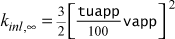
This calculation is presented in the external flows: initial profiles section of this website. Note: for laminar flows and transitional or fully turbulent flows using the mixing length turbulence model , tuapp must be set =0 because of the way the TEXSTAN's input file read structure is designed.

For internal flows the variable is used to establish the initial value of the turbulence kinetic energy, k, at the entrance to the pipe or channel. The value k_inl is computed using the input variables tuapp and the flow mass-averaged (mean) velocity and the definition
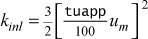
This calculation is presented in the internal flows: initial profiles section of this website. Note: for laminar flows and transitional or fully turbulent flows using the mixing length turbulence model , tuapp must be set =0 because of the way the TEXSTAN's input file read structure is designed.

twall: For internal flows this variable is the initial value of the wall temperature in units of ºC or K, SI (or) ºF or ºR, US/Eng at x = xstart. It is primarily used to create a flat inlet temperature profile by setting its value equal to tref. The use of twall is presented in the internal flows: initial profiles section of this website. Note: if only the momentum equation is being solved, twall must be set =0 because of the way the TEXSTAN's input file read structure is designed.

U top of page

ubE(m)

x-component velocity array at the E-surface (units of m/s, SI; ft/s, US/Eng)

ubE(m)	kgeom	definition
= u_∞(x)	= 1,2,3	free stream velocity boundary condition at the E-surface
= 0.0	= 4,5,6,7	no-slip boundary condition at the E-surface

For external flows, it is imperative that u_∞ (x) be smooth because it is differentiated and formulated into a pressure gradient, dP/dx, using Euler's streamline-direction equation for inviscid fluid motion, ignoring axial-direction surface curvature
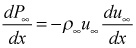
The velocity distribution can be checked using the k8=36 diagnostic check, as discussed in the overview: bc smoothness section of this website. The analysis occurs as soon as TEXSTAN is started, and then TEXSTAN is terminated to permit the user to analyze the results. Briefly, TEXSTAN's k8=36 analysis procedure is as follows:

curvefit the ubE(m)array using TEXSTAN's pressure-gradient forming spline interpolation routine
evaluate the array at 250 x locations over the interval from xstart to xend
formulate the free stream velocity, pressure gradient, acceleration parameter, and Mach number distribution at each of these 250 locations

Note that this 250-point analysis becomes a snapshot of what TEXSTAN actually obtains for the local pressure gradient as it integrates in the x direction. In refining this procedure we have found that the 250 point analysis permits observing fast-changing pressure gradients in the leading-edge region of (say) the suction side of a turbine airfoil.

The user can then plot the pressure gradient array in analysis file tex_edge.txt and check for smoothness. This procedure will help the user be sure their free stream velocity array, ubI(m), is differentially smooth. If it is not smooth, then some type of numerical smoothing software, perhaps using a least-squares method, needs to be used to smooth the array. Once the velocity array is smoothed, it needs to be rechecked for smoothness. Once again, it is imperative the pressure gradient distribution is smooth, especially for flow over turbine airfoils (blades and vanes), and the user can not be assured the pressure gradient is smooth by examination of the velocity profile itself.

ubI(m)

x-component velocity array at the I-surface (units of m/s, SI; ft/s, US/Eng)

ubI(m)	kgeom	definition
= 0.0	= 1,2,3 and 6,7	no-slip boundary condition at the I-surface
= 0.0	= 4,5	symmetry line boundary condition at the I-surface

V top of page

vapp

approach velocity (units are m/s, SI; ft/s, US/Eng)

vapp	ktmtr	approach velocity for use with Tu in transition models
= 0.0	= 0, 1, 4	not required if no transition model, or for abrupt or Kays/Crawford sine model
= V_app	= 2, 3, 5	required for two-eqn transition (ktmu=23), Abu-Ghannam/Shah, and Mayle models

vapp	ktmu	approach velocity for use with Tu in setting initial turbulence kinetic energy
= 0.0	= 1-8	not required for mixing-length models unless required for a transition model
= V_app	= 11, 21-24	required for one-equation and two-eqn turbulence models

This variable is only used for external flows as an input parameter to some turbulence models, or to establish the initial value of the turbulence kinetic energy, k_inl,∞ , at edge of the boundary layer for one- and two-equation turbulence models, computed using the input variables tuapp and vapp and the definition

These two variables are presented in the external flows: initial profiles section of this website. Note: for laminar flows and for transitional or fully turbulent flows that do not require vapp, it must be set =0 because of the way the TEXSTAN's input file read structure is designed.

viscoc

Fluid dynamic viscosity (units are (N-s)/m² or (Pa-s), SI; lbm/(s-ft), US/Eng)

viscoc	kfluid	dynamic viscosity
= (input variable)	= 1	μ supplied by user
= 0.0	= 2,4,6,8,16	TEXSTAN interpolates from table lookup
= 0.0	= 13,14,15	TEXSTAN computes from Sutherland law
= 0.0	= 15	TEXSTAN Computes from Sutherland law and (ρμ)=constant model

The user needs to pay special attention to the required US/Eng units for dynamic viscosity. This issue is the classic problem of lb-mass and lb-force for the US/Eng units. Briefly, for U.S. Customary units (sometimes called British or English units), lb-force is considered in TEXSTAN as a secondary unit and lb-mass is considered the primary unit for all physical variables. The force-mass conversion factor from Newton's Second Law, g_c is built into all equations within TEXSTAN to insure consistency of units within each equation. The discussion of units can be found in the overview: units section of this website.

W top of page

X top of page

x(m): The x(m) array defines all boundary condition locations (units are m, SI; ft, US/Eng), where the variable x is used to denote the flow direction, measured along the I-surface. This coordinate is sometimes referred to as an intrinsic coordinate, or a streamline coordinate. The x(m) array contains the locations where all boundary condition information is specified. In this array, the m subscript ranges 1 ≤ m ≤ nxbc where the variable nxbc has already been set. Recall that nxbc must be > 2. The x(m) array brackets the values of xstart and xend. It is permissible for xstart to be > x(1) and xend to be < x(nxbc). Note that it is ok to have x(1) < 0. The upper limit on this array (nxbc) has been set in TEXSTAN to be 101 points.

xend: x-location to stop integration, xend ≤ x(nxbc); (units are m, SI; ft, US/Eng).

xstart

x-location to start integration, xstart ≥ x(1); (units are m, SI; ft, US/Eng). Boundary conditions are defined over the interval defined by the array x(m), and xstart must be ≥ x(1).

For external flows there is a special relationship between xstart and the virtual origin, and it is discussed in detail in the external flows: integration control section of this website. The initial value of the x-Reynolds number is defined as rex=(xstart-xvo)*uinf*rhoc/viscoc. Here, the uinf value comes from interpolation of the ubE(m) table at x=xstart. The virtual origin is by default set =0, or it can be input using k1=1 and gxx. For kstart=0,10 xvo is computed from the input velocity profile. For kstart =5, xvo is =cxx. Note that it is permissible to have xstart be negative. There is no virtual origin for internal flows.